Baseline data for the Pinnace Channel Aquaculture Site
Noel Coleman, Andrew Longmore and Brian Cohen
Marine and Freshwater Resources Institute
Report No.34
March 2001
ISSN: 1328-5548
ISBN: 1 74106 342 6
Preferred way to cite this publication:
Coleman, N., Longmore, A., and Cohen, B. (2001). Baseline data for the Pinnace Channel Aquaculture Site. Marine and Freshwater Resources Institute Report No. 34. (Marine and Freshwater Resources Institute: Queenscliff).
Summary
A baseline survey of physical and biological characteristics of the proposed Pinnace Channel Aquaculture Site has been carried out.
The sediment is predominantly of very fine sand with some areas of fine sand. The mud content of the sediment ranges from approximately 8 – 40 %. Sediment characteristics are related to depth with grain size becoming smaller and mud content higher as depth increases.
Sediment organic carbon content correlated strongly with depth. Stable isotopes of carbon (13C/12C) and nitrogen (15N/14N) indicated that macrophytes (most likely seagrass) were the major source of organic matter in the study area. Fresh phytoplankton did not appear to make a significant contribution, and we conclude that the potential future impact of both passive and active-feeding aquaculture should be easy to detect.
Samples of benthic infauna produced 4,307 individuals and 137 species. Species diversity and evenness at the sample sites were relatively high. The distribution of the fauna was influenced by depth. The number of individuals and species per sample decreased with depth while evenness increased. Pattern analysis produced two station groups, one containing stations from 20 m of water or less and one containing stations from more than 20 m of water. The species contributing most to the station groupings were either absent from or were conspicuously less abundant at the deeper stations. The species collected were those that have been recorded in previous surveys of Port Phillip, and the fauna of the Pinnace Channel Aquaculture Site appears to be fairly typical of the fauna found generally in that part of the bay.
Benthic oxygen, carbon and nutrient fluxes at three sites were similar to those measured previously in central Port Phillip Bay. Calculations of denitrification efficiency (a measure of the ability of the system to transform biologically available N to inert N2 gas) indicated denitrification in the study area was much less efficient than in most other areas of Port Phillip Bay. This may be a consequence of a low rate of supply of organic matter to the sediment, but depends strongly on the source of labile organic matter.
Video analysis showed that sediment characteristics and bottom relief varied across the surveyed area particularly in relation to depth. Sediments in less than 20m were sandy and the bedform was dominated by callianassid mounds. Sediments in more than 20m of water were muddy and the sediment profile was flat. Fourteen epifaunal species were identified from the video footage and the ascidian Pyura stolonifera was the most commonly recorded species. Abundances of epifauna were generally low and the abundance of many species varied between the shallow, sandy sediments and the deeper, muddy sediments. The distribution and abundance of epifauna across the Pinnace Channel Aquaculture Site, and their distribution with depth, is typical of the 'intermediate sediments' epifaunal community found in Port Phillip Bay.
1 - Introduction
The Fisheries Act (1995) specifies that each Marine Aquaculture Fisheries Reserve is developed and managed according to a specific Management Plan. An important component of every Management Plan is environmental management and monitoring. Environmental monitoring may involve two phases: an initial baseline study, followed by continued monitoring to assess environmental impacts (if any) within the aquaculture area. The specific baseline and monitoring work required may vary according to the particular area under consideration and the species to be cultured but is likely to include: a review of existing data relevant to the area under consideration, determination of bathymetry and bottom type, determination of sediment characteristics, surveys of bottom communities, organic carbon content, investigation of nutrient fluxes and of stable isotope ratios (Neil Hickman, Marine and Freshwater Resources Institute, Indicative Environmental Guidelines for the Preparation of Marine Aquaculture Management Plans).
A new aquaculture zone has been recommended for an area adjacent to the Pinnace Channel in southern Port Phillip. In response to management requirements, a baseline survey was undertaken and consisted of six components:
- a review of existing relevant data
- collection of bathymetric data
- measurement of sediment particle size and of carbon and nitrogen stable isotope concentrations
- preliminary investigation of the infauna and archiving of samples for future reference.
- estimation of benthic oxygen consumption, nutrient fluxes and denitrification efficiency.
- video survey of the bottom
Background environmental information, the first component of the study, was reported in Hickman and Coleman (1998) and the second component, the bathymetry, is reported in Barry and Bailey (2001).
The video survey presents a view of the entire area as it is now while the remaining components of the study were integrated so that determination of sediment type, stable isotope ratios, infaunal community structure and benthic fluxes were all carried out at the same sample sites. Furthermore, they were chosen on the basis that comparison of the present results with those from any future studies should readily indicate whether or not environmental changes have occurred. Change is a normal feature of the natural environment, even in the absence of human activity, and any future changes to the environment in the Pinnace Channel aquaculture area need not necesssarily result from aquaculture activity. However, for the baseline studies reported here a theoretical framework exists within which it should be possible to determine whether any observed changes do result from aquaculture activities in the area rather than from naturally occurring patterns of seasonal or annual change. The framework underpinning the relevance of these studies and the studies themselves are discussed in the following sections.
2 - Survey Area and Design
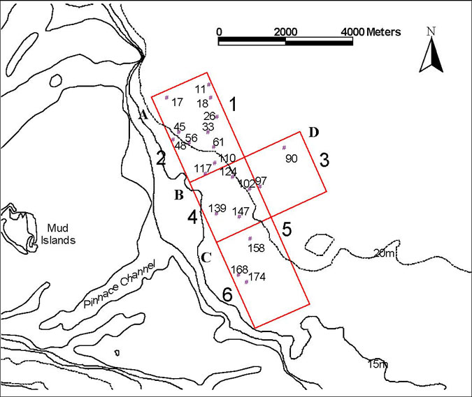
The Pinnace Channel Aquaculture Site consists of three segments, A – C in figure 2.1. Aquaculture will be permitted in zones A and C and zone B is to provide a control site for use in future monitoring studies. Sample stations were randomly allocated to each zone. There is very little water greater than 20 m in depth in the control area, whereas there is a large area with water greater than 20 m depth in aquaculture zone A. Therefore, for the purposes of the baseline survey, samples were taken from water of greater than 20 m depth from an area adjacent to the control segment (B) of the aquaculture zone. The additional area from which these samples were taken is shown as area D in figure 1. In addition, the aquaculture zone, and additional control area, were divided into six segments on the basis of depth. Segments 1, 3 and 5 are those with water of 20 m or more in depth and segments 2, 4 and 6 are those with water of less than 20 m depth (figure 2.1).
In all, 180 stations were randomly allocated to zones A to D (fig. 2.1). One station was selected at random from each of zones A to C for benthic flux measurements (stations 26, 139 and 168 in figure 2.1). After the measurements had been made, divers used suction samplers to sample sediment from an area of 0.1m2 from under and around the benthic chambers (which have an area of 0.07m2). Sediment grain size was determined, stable isotope ratios were measured and the infauna was removed, identified and counted. All the other stations were sampled with a Smith-McIntyre grab, which samples an area of 0.1m2. A subsample of 17 stations, encompassing each of the areas sampled, was selected, grain size was determined, stable isotope ratios were measured and the invertebrate fauna was removed, identified and counted. The remaining samples are archived at the Marine and Freshwater Resources Institute. In total 20 stations were sorted for the baseline survey (the 3 stations monitored for benthic fluxes + the additional subsample of 17) but no stations from segment 5 (water of 20 m+ depth from aquaculture zone C) were included in the survey because of the small extent of this segment.
Sampling and experimental work was carried out between 16 June and 2 September 1999.
3 - Sediment Grain Size and Stable Isotope Analysis
3.1 - Introduction
Sediment characteristics, particularly mean grain size, sorting (a measure of the spread of grain sizes around the mean) and the proportion of mud all influence the abundance and distribution of infaunal species. Studies within Port Phillip (Currie and Parry 1999) show that geographical location within the bay, as well as sediment type, also influence species richness and community structure. An understanding of all of these relationships is important in interpreting infaunal data from the Pinnace Channel site as it is now and in the assessment of any future changes in the fauna and the factors that may be causing them.
Organic carbon content may give some indication of the supply of organic matter to the sediment (and therefor of susceptibility of the sediment to anoxia) but gives no indication of the source of the organic matter. The stable isotope composition of organic matter in the aquaculture zone can be used (with appropriate end-members) to identify the source(s) of organic matter to the sediment. For example, if shellfish cultivation led to an increase in the deposition of pseudofaeces in the area, or finfish culture resulted in the accumulation of uneaten fish pellets, both of these could be detected by the analysis of stable isotope composition.
Butler and co-workers (CSIRO Huon Estuary Study Team. 2000) used stable N and C isotope analyses to show the area of impact of waste food from fish farms in the Huon Estuary, and recommended the method as one of great promise. The signal from fish food could be separated quite clearly from those for seagrass, marine algae and terrestrial plants. In contrast, while concentrations generally declined with distance near fish cages, organic carbon content of the Huon sediments was quite variable, and related more to sediment grain size than proximity to fish farms.
3.2 - Materials and Methods.
Survey design and the collection of samples has already been described.
Sediment grain size was determined by settling tube analysis (George and Black 1991). Particle size is not measured directly but is computed indirectly by measuring the rates at which particles fall through a known depth of water.
The settling tube used consists of a 1.9 m long perspex tube of 0.4 m internal diameter filled with salt water whose temperature and salinity are measured. The sediment sample is released at the top of the column by a motorised spinning disc which spreads sediment uniformly across the water column. Sediment settling near the base of the column is collected on a plate connected to an electronic balance and the weight of sediment settling on to the plate is transmitted to a computer. Particle size is calculated using the relationship between settling velocity and sphere radius determined by Gibbs et al (1971).
The two main causes of error in settling tube analysis are wall effects and clumping of sediment. These are overcome in the system used by having a tube of 0.4 m diameter to minimise wall effects; by making the settling plate considerably smaller than the tube diameter so that materials near the walls are not collected; by using a spinning disc release system that provides minimal turbulence; and by having a sample size in the range 1 – 10 g so as to minimise grain/grain interaction and sample error. In addition, the system is calibrated by measuring the settlement of glass beads of known size and density.
Sediments from 20 of the 160 sample sites were stored in plastic ("Whirlpak") bags, frozen and freeze-dried. A subsample of sediment from each sample site was treated with HCl to remove inorganic carbon and then rinsed thoroughly with distilled water and oven-dried. The subsamples were then weighed into tin foil capsules, and volatilised in a GC mass spectrometer, which measured the absolute concentrations of organic carbon and nitrogen, and relative abundances of the stable isotopes 13C, 12C,15N and 14N. Relative abundances are expressed as the difference, in parts per thousand, between stable isotope concentration ratios measured in the samples and those of standard materials (Pee-Dee belemnite for C and atmospheric N2 for N).
3.3 Results
The mean grain size (Table 3.1) of sediment analysed from the Pinnace Channel Aquaculture Site is predominantly that of very fine sand (0.06 – 0.125 mm) with a few stations having a mean grain size of fine sand (0.125 – 0.25 mm). Mud content ranged from 8% to 40%.
The percent sand and mud in the sediment and the mean grain size were all clearly related to depth, with sediments becoming muddier and of smaller mean grain size with increasing depth (figure 3.1).
Table 3.1. Location and sediment characteristics for stations sampled at the Pinnace Channel Aquaculture Site. Sorting is a measure of the spread of grain sizes around the mean.
| Area | Station |
Depth (m) | Location |
Mean grain size (mm) | Sorting | Sand (%) | Mud (%) |
|---|---|---|---|---|---|---|---|
| 1 | 11 | 25 | 38°14.169′S, 144°49.978′E | 0.06 | 0.41 | 59.93 | 40.07 |
| 17 | 23 | 38°14.361′S 144°49.117′E | 0.12 | 0.43 | 86.80 | 13.20 | |
| 18 | 25 | 38°14.380′S 144°50.019′E | 0.07 | 0.42 | 73.36 | 26.64 | |
| 26 | 24 | 38°14.691′ 144°50.138′E | 0.08 | 0.33 | 67.26 | 32.74 | |
| 33 | 25 | 38°14.934′S 144°49.952′E | 0.09 | 0.38 | 75.83 | 24.17 | |
| 45 | 22 | 38°14.923′S 144°49.345′E | 0.12 | 0.52 | 91.66 | 8.34 | |
| 56 | 22 | 38°15.105′S 144°49.558′E | 0.12 | 0.43 | 86.8 | 13.20 | |
| 61 | 24 | 38°15.175′S 144°50.055′E | 0.13 | 0.41 | 86.65 | 13.35 | |
| 2 | 48 | 18 | 38°15.049′S 144°49.219′E | 0.13 | 0.47 | 89.02 | 10.98 |
| 110 | 18 | 38°15.441′S 144°50.069′E | 0.10 | 0.34 | 77.48 | 22.52 | |
| 117 | 18 | 38°15.605′S 144°49.875′E | 0.13 | 0.46 | 91.87 | 8.13 | |
| 3 | 90 | 23 | 38°15.213′S 144°51.499′E | 0.07 | 0.34 | 67.27 | 32.73 |
| 97 | 23 | 38°15.830′S 144°50.992′E | 0.08 | 0.42 | 72.85 | 27.15 | |
| 102 | 20 | 38°15.869′S 144°50.774′E | 0.12 | 0.50 | 92.34 | 7.66 | |
| 124 | 20 | 38°15.666′S 144°50.425′E | 0.13 | 0.36 | 81.95 | 18.05 | |
| 4 | 139 | 17 | 38°16.253′S 144°50.075′E | 0.11 | 0.44 | 88.64 | 11.36 |
| 147 | 18 | 38°16.312′S 144°50.550′E | 0.14 | 0.34 | 89.81 | 10.19 | |
| 6 | 158 | 18 | 38°16.676′S 144°50.762′E | 0.11 | 0.40 | 84.87 | 15.13 |
| 168 | 19 | 38°17.252′S 144°50.497′E | 0.14 | 0.52 | 91.75 | 8.25 | |
| 174 | 18 | 38°17.369′S 144°50.663′E | 0.14 | 0.45 | 90.96 | 9.04 |
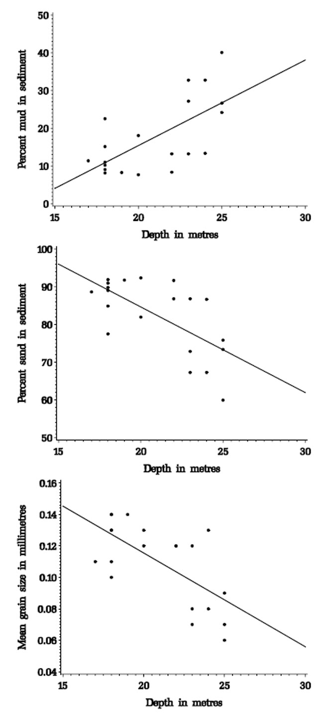
Figure 3.1. Correlations between depth and sediment characteristics for sediment samples from the Pinnace Channel Aquaculture Site. Percent mud in sediment= -29.99 + 2.27 x depth; r2 = 0.44, p = 0.0015 Percent sand in sediment= -129.99 – 2.27 x depth; r2 = 0.44, p = 0.0015 Mean grain size in millimetres = 0.23-0.006 x depth; r2 = 0.44, p = 0.0015
There was considerable variation between sites in carbon and nitrogen concentrations and stable isotope relative abundances (Table 3.2). Correlations between environmental characteristics were carried out using the Correlation procedure of SAS (Statistical Analysis Software Version 8), with square-root transformed variables. Where two or more environmental factors were correlated, partial correlation was used to determine which factor was most significantly correlated.
δ15N correlated with sand content. δ13C correlated with %N, %C, grain size, sand and mud by virtue of their correlations with depth; %C correlated so strongly with depth that controlling for %C rendered the relationship between δ13C and depth nonsignificant.
Table 3.2. Total nitrogen, total carbon and stable isotope ratios for organic matter from 20 sites near the Pinnace Channel. Note that no samples from segment 5 were analysed.
| Segment | Site | Depth (m) | %N | %C | δ 15N ppt | δ 13C ppt |
|---|---|---|---|---|---|---|
| 1 | 11 | 25 | 0.175 | 1.648 | 0.49 | -17.53 |
| 1 | 17 | 23 | 0.138 | 1.713 | 4.12 | -12.20 |
| 1 | 18 | 25 | 0.167 | 1.437 | 4.51 | -19.21 |
| 1 | 26 | 24 | 0.131 | 2.207 | 1.67 | -9.36 |
| 1 | 33 | 25 | 0.106 | 2.353 | 0.80 | -7.42 |
| 2 | 45 | 22 | 0.110 | 3.936 | 3.84 | -3.73 |
| 2 | 48 | 18 | 0.092 | 3.434 | 4.32 | -3.82 |
| 2 | 56 | 19 | 0.112 | 3.974 | 1.19 | -3.58 |
| 2 | 61 | 24 | 0.116 | 2.368 | 5.32 | -7.33 |
| 3 | 90 | 23 | 0.189 | 1.469 | 2.06 | -21.07 |
| 3 | 97 | 23 | 0.127 | 1.441 | -0.93 | -14.57 |
| 3 | 102 | 20 | 0.117 | 2.337 | 6.17 | -8.05 |
| 4 | 110 | 18 | 0.141 | 2.549 | 4.50 | -8.15 |
| 4 | 117 | 18 | 0.063 | 5.606 | 2.22 | -0.78 |
| 4 | 124 | 20 | 0.117 | 3.614 | 2.50 | -4.50 |
| 4 | 139 | 17 | 0.075 | 5.140 | 3.72 | -1.24 |
| 6 | 147 | 18 | 0.073 | 3.856 | 2.38 | -1.80 |
| 6 | 158 | 18 | 0.095 | 4.322 | 1.80 | -2.87 |
| 6 | 168 | 19 | 0.073 | 5.225 | -4.81 | -1.18 |
| 6 | 174 | 18 | 0.070 | 5.304 | 5.09 | -1.08 |
| Mean | 0.114 | 2.55 | 3.20 | -7.47 | ||
| ±S.D. | 0.036 | 2.52 | 1.42 | 6.36 |
However, there were no statistically-significant differences between segment means (Table 3.3) for %N, δ15 N or δ13C. Statistically-significant differences were found between segments for %C, by which segments could be further consolidated into two groups. The first group is samples from segments 1 and 3, with low carbon (1.8%), high nitrogen (0.14%), low δ15N (2.4 ppt) and depleted δ13C (-14 ppt). The second group is from segments 2 , 4, and 6, with high carbon (4%), low N (0.1%), high δ15N (3.4 ppt) and enriched δ13C (-4 ppt). Segments 1 and 3 are deeper than the other segments, re-emphasizing the relationships with depth identified above.
Table 3.3. Mean abundances (± 1 S.D.) for each segment.
| Segment | %N | %C | δ15N | δ13C |
|---|---|---|---|---|
| 1 | 0.143 ± 0.028 | 1.871 ± 0.39 | 2.32 ± 1.878 | -13.14 ± 5.10 |
| 2 | 0.108 ± 0.011 | 3.428 ± 0.75 | 3.67 ± 1.763 | -4.62 ± 1.81 |
| 3 | 0.144 ± 0.089 | 1.749 ± 0.51 | 2.43 ± 3.564 | -14.56 ± 6.51 |
| 4 | 0.099 ± 0.036 | 4.227 ± 1.41 | 3.24 ± 1.135 | -3.67 ± 3.42 |
| 6 | 0.078 ± 0.012 | 4.677 ± 0.71 | 1.12 ± 4.202 | -1.73 ± 0.82 |
3.4 - Discussion
When compared to stable isotope abundances observed elsewhere (Table 3.4), it is clear that phytoplankton do not form a significant proportion of the organic supply to the sediments in the study area. If phytoplankton were important, we would expect δ13C abundances of –18 to –22. Sediments from group 1 (segments 1 and 3) have stable carbon signatures similar to seagrass (~-12 to –16). Sediments from the other groups are so enriched in 13C (less negative) compared to typical primary producers found elsewhere (Table 3.4) that we could conclude the organic matter has passed through detrital loops several times, with a fractional enrichment in 13C on each cycle. From this argument, the organic material at most sites is therefore not fresh, but substantially degraded. An alternative argument is that seagrasses on the Sands have a much higher (less negative) 13C signal than in most other studies. For example, Fry and Parker (1979) found 13C abundances as high as –3 ppt for some seagrasses in a Texas estuary. Under high light conditions, such as we might expect at the Sands, seagrasses may be enriched in 13C by 3-4 ppt (Grice et al. 1996). Another alternative argument is that the sediments contained a substantial proportion of carbonate, which has a 13C signature close to zero. However, significant effort was put into removing carbonate from the samples (see Method), and this is unlikely.
Without measurement of the stable isotope concentrations in the likely sources of organic matter to the study area, it is not possible to be more definitive about likely sources. However, the stable nitrogen relative abundance was within the range observed elsewhere for macrophytes and algae growing under oligotrophic conditions (Grice et al. 1996).
If passive aquaculture leads to the increased deposition of phytoplankton debris, such a signal should be clearly indicated by a more negative 13C ratio. Pelletised food based on imported fish meal has an isotopic signature of δ13C ~ -23 and δ15N ~ 14 (M. Burford, CRC for Aquaculture, pers. Comm.). The impact of undigested artificial food and food residue should therefore also be easily observed in the stable isotope relative abundances. However, to improve the likelihood of detecting change, once a specific aquaculture enterprise is assigned an area, all sediment samples (~30) from within the appropriate segment should be analysed for stable isotope concentration, and these analyses then used to determine the mean and standard deviation for the segment.
Table 3.4. Mean stable isotope relative abundances in different source materials.
| Source | δ13C | δ15N | Reference |
|---|---|---|---|
| Florida lake sediments | -24 | 2.7 | Gu et al. (1996) |
| Particulate organic matter | -28 | 4.9 | Hobson et al. (1995) |
| Corner Inlet sediment | -18.7 | Nichols et al. (1985) | |
| Sea ice algae | -18.6 | 8.3 | Hobson et al. (1995) |
| Fast-growing diatoms | -15 to –19 | Fry and Wainright (1991) | |
| Slow-growing diatoms | -21 to –25 | Fry and Wainright (1991) | |
| Marine phytoplankton | -22 | France (1995) | |
| Torres Strait plankton | -21.8 | Fry et al. (1983) | |
| Marine benthic algae | -17 (but one sample –4) | France (1995) | |
| Seagrasses | -11 (range -23 to –3) | Hemminga and Mateo (1996) | |
| Benthic seagrasses (N. Qld) | -8.8 | Fry et al. (1983) | |
| Seagrasses (Qld) | -11 | 2-4 | Loneragan et al. |
| Heterozostera | -12 | Fenton and Ritz (1988) | |
| Western Port seagrasses | -11.7 | 3.9 | Boon et al. (1997) |
| Western Port seagrass epiphytes | -17.9 | 4.6 | Boon et al. (1997) |
| Western Port Enteromorpha | -19 | 8 | Boon et al. (1997) |
| Western Port mangroves | -26 | 3 | Boon et al. (1997) |
| Western Port saltmarsh plants | -26 | 3 | Boon et al. (1997) |
| Macroalgae (N. Qld) | -12.5 | Fry et al. (1983) | |
| Epiphytic algae (N. Qld) | -13.3 | Fry et al. (1983) |
4 - Infaunal Benthic Invertebrates
4.1 - Introduction
There is an extensive literature on the use of benthic infaunal communities for environmental monitoring. A major concern in areas where aquaculture is conducted is that of nutrient or organic enrichment, which may, for example, arise through the accumulation of pseudofaeces where shellfish culture occurs or through organic wastes associated with fish farming (Henderson and Ross 1995; Kaiser et al. 1998). Environmental changes associated with nutrient enrichment are also found in areas subject to sewage discharge and have been well studied (Zarkanellas 1979; Swartz et al. 1986; Ismail 1992).
In extreme cases, where there is very high build up of organic material in the sediment, bacterial decomposition of this material may lead to oxygen depletion and the elimination of the invertebrate infauna. Where the build-up of organic material is less, the effect may be to produce a community in which the number of individuals is higher but the number of species is lower than in non-impacted areas. This pattern arises because species unable to withstand the environmental changes associated with enrichment are eliminated while other, opportunistic species benefit from the changes and increase greatly in numbers. The combination of high numbers of individuals and low numbers of species results in a community which is heavily dominated by one or a few species and in which species richness and diversity are low.
4.2 - Materials and Methods
Survey design and the collection of samples has already been described.
In the laboratory the samples for faunal analysis were passed through a 1 mm mesh sieve. Material retained on the sieve was placed under a low-powered dissecting microscope for sorting and the animals were removed from the samples, identified and counted. Identifications were made by comparing individuals against reference material verified by staff at Museum Victoria.
The total number of individuals and species per station were determined. The Shannon-Weiner species diversity index, H' (where H' = -∑pIlogepI where pI is the proportion of individuals in the ith species), was calculated for each station. Evenness, J', was calculated using Pielou's formula (J' = H'/loges where s is the number of species per station).
Correlations between environmental and faunal characteristics were carried out using the Correlation procedure of SAS (Statistical Analysis Software Version 7). Where two or more environmental factors were correlated with the fauna, partial correlation was used to determine which factor was most significantly correlated with the fauna.
The General Linear Modelling procedure of SAS was used to compare faunal characteristics between depths. General Linear Modelling is similar to analysis of variance but is less influenced by differences in the size of the samples being compared. Before mean values were compared Bartletts test was used to check for homogeneity of variance. Where necessary transormation of the data was used to produce homogeneity.
Pattern analysis was carried out using PATN (Belbin 1991). Analyses were carried out on the total number of individuals and species per station using both raw and transformed data. Transformation (usually by taking the logarithm, the square root or the double square root of the number of individuals per station) is carried out in order to make the spread of values (of individuals per species) more equal and prevent the analyses being dominated by the few most abundant species. The patterns generated have a stress value associated with them. Values in excess of 0.20 indicate that the patterns generated do not adequately represent the data (ie. Little reliance should be placed on the patterns generated). Below a stress value of 0.20, the lower the value the better does the pattern represent the data. Multidimensional scaling (MDS) plots were based on differences in species composition between sites calculated using the Bray-Curtis dissimilarity measure. Kruskal-Wallis values were determined to show which species contributed most to the station groups indicated by pattern analysis.
4.3 - Results
The total number of individuals sorted from the samples was 4,307 and the total number of species was 137. The number of individuals per station ranged from 54 to 519 and the number of species from 16 to 50 (Table 4.1).
Table 4.1. Community characteristics for infaunal invertebrates at the Pinnace Channel Stations.
| Station | Segment |
Depth (m) | No. of individuals | No. of species | Species diversity, H' | Evenness, J' |
|---|---|---|---|---|---|---|
| 11 | 1 | 25 | 94 | 26 | 2.80 | 0.86 |
| 17 | 1 | 23 | 139 | 25 | 2.44 | 0.76 |
| 18 | 1 | 25 | 105 | 27 | 2.75 | 0.83 |
| 26 | 1 | 24 | 54 | 16 | 2.31 | 0.83 |
| 33 | 1 | 25 | 90 | 21 | 2.52 | 0.83 |
| 45 | 1 | 22 | 116 | 21 | 2.36 | 0.76 |
| 56 | 1 | 22 | 130 | 24 | 2.56 | 0.81 |
| 61 | 1 | 24 | 117 | 24 | 2.68 | 0.84 |
| 48 | 2 | 18 | 310 | 31 | 1.89 | 0.55 |
| 110 | 2 | 18 | 311 | 45 | 2.60 | 0.68 |
| 117 | 2 | 18 | 333 | 41 | 2.44 | 0.66 |
| 90 | 3 | 23 | 60 | 24 | 2.74 | 0.86 |
| 97 | 3 | 23 | 199 | 38 | 2.89 | 0.79 |
| 102 | 3 | 20 | 214 | 30 | 2.01 | 0.59 |
| 124 | 3 | 20 | 235 | 38 | 2.61 | 0.72 |
| 139 | 4 | 17 | 353 | 50 | 2.83 | 0.72 |
| 147 | 4 | 18 | 519 | 50 | 2.81 | 0.72 |
| 158 | 6 | 18 | 227 | 29 | 2.59 | 0.77 |
| 168 | 6 | 19 | 238 | 33 | 2.17 | 0.62 |
| 174 | 6 | 18 | 463 | 45 | 2.84 | 0.75 |
The most abundant and widespread species in the samples was the polychaete Lumbrineris cf latreilli which provided 1242 (29% of the) individuals and occurred at all the stations. Only one other species, the polychaete Marphysa sp 1, occurred at all stations and this was also relatively abundant, providing 389 (9% of the) individuals. Other relatively abundant species were the crustacean Kalliapseudes sp 1 (provided 468 individuals and occurred at 18 stations), the bivalve Chioneryx cardioides (provided 208 individuals and occurred at 15 stations), the polychaete Nephtys inornata (provided 200 individuals and occurred at 19 stations), the bivalve Nucula obliqua (provided 125 individuals and occurred at 19 stations), the polychaete Maldanid sp 1 (provided 102 individuals and occurred at 16 stations) and the exotic bivalve Corbula gibba (provided 92 individuals and occurred at 17 stations). The majority of species may be regarded as relatively uncommon. Ninety two species were each represented by less than 10 individuals and 69 species occurred at only one or two stations.
Species diversity ranged from 1.89 to 2.89 and evenness from 0.55 to 0.86 (Table 4.1). The generally high values for evenness show that the number of individuals per station was fairly evenly divided amongst the species present, with no one or two species being overwhelmingly dominant. At station 48, which had the lowest evenness (0.55), the most abundant species (Kalliapseudes sp 1) provided 47% of the individuals while at stations 11 and 90, which had the highest evenness (0.86), the most abundant species provided respectively 21% and 23% of the total individuals per station.
The number of individuals, the number of species and evenness per station are all clearly related to depth (Figure 4.1). However, they are also related to a range of other environmental factors which are themselves interrelated (Tables 4.2 and 4.3) and partial correlation was used to determine which factors were most significantly correlated with community characteristics.
The number of individuals per stations was significantly correlated with depth, grain size, sand and mud (Table 4.2). Partial correlations suggest that the most important of these characteristics in relation to the number of individuals is depth. The correlation between number of individuals and depth remained significant when the influence of the other variables was removed, but removing the influence of depth rendered correlations between individuals and grain size, sand and mud non significant. Similarly, correlations between the number of individuals and the various measures of nitrogen and carbon became non-significant when the effects of depth were removed.
The number of species per station was significantly correlated with depth, and with the percentages of nitrogen and carbon in the sediment. Correlations with nitrogen and carbon became non-significant when the effects of depth were removed, but the correlation with depth remained significant when the influences of nitrogen and carbon were removed.
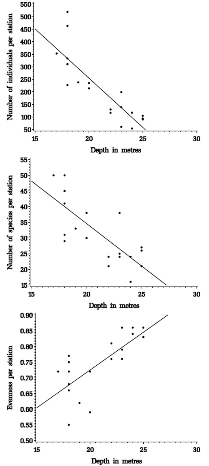
Figure 4.1. Correlations between depth and faunal characteristics for stations from the Pinnace Channel Aquaculture Site.
Number of individuals per station -= 1039 – 39 x depth; r2 = 0.72, p = <0.0001
Number of species per station -= 88.71 – 2.71 x depth; r2 = 0.58, p = <0.0001
Evenness per station -= 0.244 + 0.024 x depth; r2 = 0.56, p = 0.0002Species
diversity was negatively correlated with sorting.
Evenness was significantly correlated with depth, grain size, sorting, sand, mud and some measures of nitrogen and carbon. As with the other correlations between environmental and community characteristics, depth appeared to be the most important factor. The correlation between depth and evenness remained significant when the effects of the other variables, singly or in combination, were removed but removing the effect of depth rendered correlations between evenness and all but one of the other environmental variables non-significant. The exception was the correlation between evenness and sorting which remained significant when the effects of depth were removed.
Table 4.2. Correlations between faunal characteristics and environmental characteristics at the Pinnace Channel stations. Upper figure is the Pearson Correlation Coefficient and lower value is the probablity. Blank spaces in the table indicate that no significant correlation was found.
| No. of individuals | No. of species | Species diversity, H' | Evenness, J' | |
|---|---|---|---|---|
| Depth (m) |
-0.85 <0.0001 |
-0.76 <0.0001 |
0.75 0.0002 | |
| Mean grain size (mm) |
0.63 0.003 |
-0.63 0.003 | ||
| Sorting |
-0.48 0.03 |
-0.52 0.02 | ||
| Sand (%) |
0.57 0.008 |
-0.68 0.001 | ||
| Mud (%) |
-0.57 0.008 |
0.68 0.001 | ||
| %N in the sediment |
-0.71 0.0005 |
-0.51 0.02 |
0.56 0.01 | |
| δ 15N | ||||
|
%C in the sediment |
0.64 0.002 |
0.51 0.023 |
-0.48 0.03 | |
| δ 13N | 0.64 |
-0.55 0.01 |
Table 4.3. Correlations between environmental variables at the pinnace Channel stations. Upper figure is the Pearson Correlation Coefficient and lower value is the probability. There were no correlations between δ 15N and the other environmental variables measured.
Table 4.3. Correlations between environmental variables at the pinnace Channel stations.
| Depth | ||||||
| Grain size |
-0.66 0.0015 | |||||
| % sand |
-0.66 0.0015 |
0.92 <0.000` | ||||
| % mud |
0.66 0.0015 |
-0.92 <0.000` |
-1.00 <.0001 | |||
| %N |
0.71 0.0005 |
-0.83 <0.0001 |
-0.80 <0.001 |
0.80 <0.0001 | ||
| %C |
-0.77 <0.0001 |
0.72 0.0004 |
0.71 0.0004 |
0.71 0.0004 |
0.87 <0.0001 | |
| δ 13C |
-0.73 0.0002 |
0.84 <0.0001 |
0.80 <0.0001 |
0.80 <0.0001 |
0.94 <0.0001 |
0.89 <0.0001 |
| Depth | Grain size | % sand | % mud | % N | % C | |
Because the distribution of the fauna is clearly related to depth, and because an obvious feature of the Pinnace Channel Aquaculture Site is that it is divided by the 20 m depth contour, mean values per station for individuals, species, species diversity and evenness were compared between stations from 20 m or less depth and those from deeper than 20 m (Table 4.4).
Table 4.4. Comparison of mean values for number of individuals, number of species, species diversity and evenness per station between stations from 20m or less in depth and stations from more than 20m in depth. S, difference is significant (probability is shown in brackets); NS, difference is not significant. Comparison of number of individuals was done on logged data but actual values are shown.
| Mean value per station for: | Station Depth | Significance | |
|---|---|---|---|
| 20 m or less | > 20m | ||
| Number of individuals | 320 | 110 | S (p = <0.0001) |
| Number of species | 39 | 25 | S (p = 0.0002) |
| Species diversity, H' | 2.48 | 2.61 | NS |
| Evenness, J' | 0.68 | 0.82 | S (p = <0.0001) |
All values except those for species diversity differed significantly between depth zones.
Pattern analyses using transformed data produced stress values in excess of 0.2, showing that the patterns were not reliable. Only pattern analysis in 3 dimensions using the raw data produced a stress value of less than 0.2 (fig. 4.2).
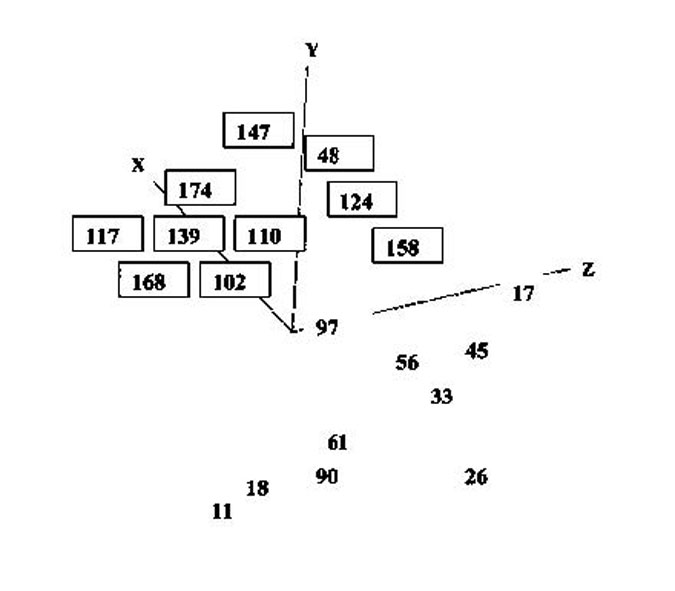
Figure 4.2. Three dimensional multidimensional scaling plot of stations from the Pinnace Channel Aquaculture Site. Stations with a border round them are those from 20 m of water or less. Stress = 0.16
The major grouping shown by the analysis is on the basis of depth, with stations from 20 m or less of water forming one group and stations from more than 20 metres of water forming the other. Within these two groups, the closeness of stations, which implies closeness of faunal similarity, is not necessarily between those stations which are spatially the closest. Thus, for example station 168 is closer in location to station 174 than to station 102, but in terms of fauna is closer to 102 than to 174.
The 22 taxa that contributed most to the differences between the two station groups (ie had the highest values of the Kruskal-Wallis statistic) were all conspicuously more widespread and abundant at the stations in shallower water (table 4.5) than at stations in water more than 20 m in depth.
Table 4.5. The twenty two species contributing most to differences between the two station groups shown by pattern analysis. K-W is the Kruskal-Wallis statistic; mean abundance is the mean value for those stations at which the species was found and % occurrence is the percentage of stations (in each group) at which each species occurred. Letters after the species names indicate that the species is a crustacean ©, echinoderm (e), nemertean (n) or polychaete (p).
| Species | K-W | Mean abundance (% occurrence) at stations | |
|---|---|---|---|
| 20 m or less in depth | More than 20 m in depth | ||
| Lumbrineris cf latreilli (p) | 13.75 | 105.8 (100) | 18.4 (100) |
| Armandia cf intermedia (p) | 11.81 | 1.8 (80) | 0 |
| Kalliapseudes sp 1 © | 11.35 | 41.5 (100) | 6.6 (80) |
| Nephtys inornata (p) | 8.96 | 14.8 (100) | 0 |
| Ampharete sp 1 (p) | 7.81 | 4.5 (60) | 0 |
| Aedicira sp 1 (p) | 7.17 | 8.8 (80) | 1.5 (20) |
| Empoulsenia sp 1 © | 6.20 | 1.6 (50) | 0 |
| Nemertean sp 7 (n) | 5.89 | 3 (70) | 0 |
| Haliophasma canale © | 5.61 | 2 (70) | 4 (10) |
| Dimorphostylis cottoni © | 5.10 | 2.3 (70) | 1.5 (20) |
| Chaetozone sp 1 (p) | 4.92 | 2.8 (80) | 1.2 (40) |
| Diplocirrus sp 1 (p) | 4.68 | 2 (40) | 0 |
| Birubius babaneekus © | 4.61 | 5.9 (70) | 1.7 (30) |
| Harmothoe sp 1 (p) | 3.88 | 1.4 (50) | 1 (10) |
| Cylindroberidid sp 1 © | 3.35 | 1 (30) | 0 |
| Leptanthura diemenensis © | 3.33 | 3.3 (30) | 0 |
| Paradexamine lanacoura © | 3.33 | 2 (30) | 0 |
| Amakusanthura olearia © | 3.33 | 1.3 (30) | 0 |
| Apseudes sp 1© | 3.33 | 2 (30) | 0 |
| Amphiura constricta (e) | 3.33 | 11 (30) | 0 |
| Halicarcinus ovatus © | 3.33 | 1.7 (30) | 0 |
| Caprella equilibra © | 3.33 | 1.7 (30) | 0 |
4.4 - Discussion
The benthic fauna of Port Phillip has been extensively studied over the last few years. In summarising previous work Poore (1992) noted that the fauna of the bay is exceptionally rich in species compared with similar embayments in other parts of the world and has a diversity of community types which are primarily correlated with sediment type. Although the fauna is diverse many species are of scattered or infrequent occurrence appearing at only a few sample stations in the studies that have been undertaken. The present survey shows that the benthos of the proposed Pinnace Channel aquaculture Site conforms to this general pattern particularly with regard to the fact that many species were represented by relatively few individuals and only occurred at one or two stations.
The distribution of fauna was clearly related to depth. Stations below 20 m depth were muddier and had finer-grained sediments than those of less than 20 m depth and the fauna was characterised by fewer individuals and species but greater evenness (ie a more even distribution of individuals amongst species) than at the shallower stations. Even though evenness differed between the deeper and shallower stations, it was generally high at all stations and it should therefore be readily apparent if nutrient enrichment from future aquaculture development were to lead to an increase in dominance of one or two opportunistic species.
Pattern analysis (using multidimensional scaling) using survey data from a bay-wide survey of the benthos carried out during 1969 – 72 showed four benthic community groupings (fig. 4.3) which could be related to the distribution of bottom sediments within the bay (Currie and Parry 1999).
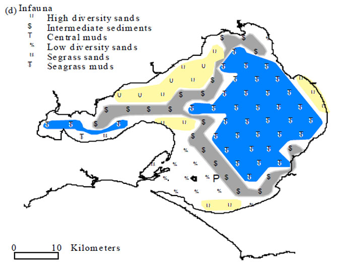
Figure 4.3. Pattern analysis of the 1969 – 72 bay-wide survey data showing major benthic community groupings. (from Currie and Parry 1999). P indicates the location of the Pinnace Channel Aquaculture Site.
The Pinnace Channel Aquaculture Site lies at the border of the 'low diversity sands' and the 'intermediate sediments' as defined by Currie and Parry (1999). Currie and Parry (1999) give (mean) numbers of species per 0.1m2 Smtih-McIntyre grab as between approximately10 and 30, though mostly between 10 and 20, for stations they define as 'low diversity sands' and between 10 and 85, but mostly within the range 20 to 60, for the stations they define as 'intermediate sediments'. Numbers of species per grab in the Pinnace Channel survey were within these ranges and, with only one grab with less than 20 species and with 10 grabs with 30 or more species, suggest that the fauna of the aquaculture zone approximates to that of the 'intermediate sediments' as defined by Currie and Parry. Values for species diversity, H', recorded in the present survey (1.89 to 2.89) were within the range of values recorded for stations in the same area surveyed between 1969 and 1973 (1.61 to 3.42) (Poore et al. 1975).
The species recorded in the survey have previously been recorded from the bay (Poore at al. 1975; Currie and Parry 1999) and in addition to looking at general faunal characteristics, such as number of species, species diversity and species dominance, future monitoring of the aquaculture zone could also utilise actual species identities and, through pattern analysis, monitor changing faunal relationships between stations. Gray et al. (1990) consider that multidimensional scaling is more sensitive than measures such as species richness, diversity and dominance in detecting impacts on benthic community structure. Changing relationships between control sites and sites where aquaculture is being undertaken, as revealed by pattern analysis, may therefore reveal the impacts, if any, of aquaculture on the benthic fauna.
Currie and Parry (1999) compared samples taken in 1991 – 1992 with those taken in 1969 – 1972 and found that there had been conspicuous changes to the fauna in the 20 years or so between the surveys. Changes could be partly explained by the introduction of exotic species into Port Phillip Bay between the surveys, but there were also marked differences between surveys in the relative abundances of the native species that were common to both. Whether the changes in the native species represent some long-term transition in the fauna of the bay or merely reflect interannual variation is not certain, but Wilson et al (1998) consider that changes in the fauna over the last 25 years are within the range encountered during a 3-year monitoring study of Port Phillip Bay benthos that was carried out during the 1970s.
In summary, the benthic infauna of the Pinnace Channel Aquaculture Site appears to be fairly typical of the benthic infauna found generally in that part of the bay. Values for number of species and species diversity per station are similar to those obtained in other surveys of the area and the species obtained are those that have been collected in previous studies. Evenness at the stations was high, showing that they are not heavily dominanted by one or two species. Community characteristics and the distributions of at least some species are clearly related to depth.
5 - Benthic Fluxes
5.1 - Introduction
As organic matter in the sediments is decomposed, its constituent elements are released for recycling. The rate with which decomposition and recycling occurs varies with a range of factors including the rate at which organic material is supplied, the nature of the material, the oxygen supply and the degree of bioturbation (mixing of the sediment by burrowing animals).
Sediments from Hobsons Bay, Werribee region and central Port Phillip Bay currently exhibit high to moderate oxygen consumption rates, and extremely efficient conversion of organic N to N2 gas, which is lost from the system. The efficiency declines as organic supply increases. No information is currently available from anywhere near the study site. Potentially, increased organic loading in the aquaculture zone could lead to a decline in oxygen concentration and denitrification efficiency, and an increased recycling of nitrogen in forms available for algal growth. The study of benthic fluxes provides a means whereby benthic oxygen consumption and denitrification efficiency may be estimated and should indicate whether any problems with oxygen depletion or nutrient recycling are likely to occur as the result of an excessive build up of organic waste.
In the context of Port Phillip Bay, the critical value to maintain is its ability to continue to denitrify the majority of the organic material reaching the sediments. The whole purpose of setting limits to the nitrogen input to the bay is to (at least) maintain the current denitrification efficiency. The major monitoring tool proposed for an ongoing PPB nitrogen monitoring program is the measurement of denitrification efficiency (Longmore 2000). The only current practical method is to use benthic chambers to do this. A range of other techniques will be investigated in the next couple of years, to see if they offer a more economical surrogate measurement of denitrification efficiency than benthic chambers do (Longmore and Gason 2001). Redox potential may be one such surrogate, but there is no published relationship between redox potential and denitrification efficiency. Port Phillip Bay appears to be "special" because of the delicate poise between oxic and anoxic micro-zones within the actively bioturbated heterogeneous sediments (Harris et al. 1996, p. 173), which a redox potential measurement is unlikely to define. Burke (1995) measured oxygen penetration depths of only 1-2 mm in most sediments from Port Phillip Bay; typical redox probes are unable to measure at such small intervals. In other areas, where denitrification may not be so important, redox potential may be a sensible indicator to use on its own, but in Port Phillip Bay it would be inappropriate to use an indicator which currently tells us nothing about the most important ecosystem function.
5.2 - Methods
5.2.1 - Sampling procedure
Benthic fluxes were estimated at three sites: 26, 139 and 168. A transparent automated benthic chamber was used to measure fluxes of oxygen, carbon dioxide, ammonium, nitrite, nitrate, phosphate and silicate. The chamber was cylindrical in shape, and covered ~0.06 m2 of sediment, trapping ~ 13 L of overlying water. The chamber had an open base that penetrated the sediment. As organic matter in the sediment is broken down, oxygen is consumed, and nutrients recycled. The rate of metabolite production or consumption (a flux) was estimated by the rate at which metabolite concentrations changed within the chamber. The chamber was stirred at a rate commensurate with bottom currents in the study area. The chamber was lowered by hand to the seafloor, and any disturbed sediment allowed to settle for two hours before a trap door closed to seal the chamber. Oxygen concentrations were measured every two minutes with a YSI salinity/temperature/dissolved oxygen probe, while carbon dioxide, ammonium, nitrite, nitrate, phosphate and silicate concentrations were measured in samples drawn automatically from the chamber at 3, 6, 9, 12, 15 and 18 hours after closure. A sample of bottom water was collected by Niskin bottle, to provide initial samples for nutrients, DO, pH and alkalinity. A spike of the inert tracer NaCl was injected into the chamber, and detected by a salinity sensor; the change in salinity was used to estimate chamber volume. Nutrient samples were filtered and frozen, while pH and alkalinity samples were stored on ice.
DO concentration in bottom water samples was measured by Winkler titration with amperometric end-point detection (Parsons et al. 1984) to a precision of 0.05 mL L-1 (about 3 M). Temperature was calibrated in the laboratory to 0.01oC against a certified Sensoren Instrument Systems digital reversing thermometer. DO molar concentration was calculated from the Ideal Gas Equation (n=PV/RT).
The inorganic nutrients ammonium, nitrite, nitrate, phosphate and silicate were measured by segmented-flow colorimetry using standard methods (Longmore et al. 1996). The estimated precision of measurement was NH4 0.1 µM, NO2 0 .02 µM, NO3 0.05 µM, PO4 0.05 µM, and SiO4 0.5 µM.
Unfiltered pH samples were kept on ice for less than six hours and analysed potentiometrically at 25oC to 0.002 pH with a Ross combination pH electrode. Great care was taken to account for electrode drift and liquid junction potential changes. The electrode was allowed to stabilise for 15 minutes in each pH buffer, and then conditioned in a saline sample for at least 10 minutes before analysing samples. Electrode potential was measured for each sample until it stabilised to a drift of less than 0.1 mV/2 min. pH was calculated from electrode potential to an accuracy of greater than 0.005 pH units.
Alkalinity was measured by Gran titration of a 4 mL filtered sample with dilute HCl solution. Samples and acid were both diluted with artificial seawater. Sample pH was brought to near pH 4.0, and then multiple standard additions made over 15 minutes, eventually reducing the pH to 3.5. A least-squares regression of pH on acid volume was used to calculate alkalinity (Hansson and Jagner 1973). Replicate titrations varied by less than 0.2%.
Total carbon dioxide concentration was calculated from pH and alkalinity, with temperature and salinity-dependent corrections for borate concentration (Dickson 1981). Carbon dioxide concentration was calculated to a precision of 5 µM.
5.2.2 - Calculation of benthic fluxes
Oxygen in the chambers could be consumed by infauna, by epifauna, by bacteria associated with the infauna, epifauna or sediment, and by re-oxidation of reduced metabolites (e.g. H2S). Oxygen concentration typically declines with time in benthic incubations (see Results below), and because the bacterial consumption rate of oxygen is first-order with respect to DO concentration, the time line is curved (Santschi et al. 1990). Different DO fluxes can therefore be calculated for different parts of the DO-time curve.
Solute concentrations were plotted for each chamber against incubation time. The period was identified during which oxygen consumption was least curved (usually the first few hours). The change in solute concentration during that period was fitted by linear least squares regression, and combined with chamber volume and sediment surface area to calculate a flux (rate of change) per unit time per unit sediment surface. These short-term fluxes were then extrapolated to a daily flux.
Denitrification efficiency (the percentage of organic nitrogen mineralised in sediments which is eliminated as N2 gas) was calculated by assuming that the majority of particulate organic matter falling to the bottom of Port Phillip Bay is of fresh diatomaceous origin, with an elemental composition of 106C:18Si:16N:1P (called the Redfield ratio). A similar calculation was made assuming seagrass was the major organic source (C:N=26 for macrophytes from nutrient-poor waters; Atkinson and Smith 1980).
5.3 - Results and discussion
Oxygen concentrations in bottom waters were close to saturation. Within the benthic chamber, nutrient concentrations increased with time, while dissolved oxygen concentrations declined (Figs 5.1, 5.2). Daily benthic fluxes (Table 5.1) were similar between sites, and also similar to previous measurements from central Port Phillip Bay (and therefore lower than fluxes estimates from Hobsons Bay and the Werribee and Corio Bay areas). When compared to the carbon dioxide fluxes, inorganic N and phosphate fluxes were all less than would be expected from the degradation of fresh diatomaceous matter, while silicate fluxes were close to expectations. Denitrification efficiency, assuming a phytoplankton source, was extremely high, at 84-87%. However, the stable isotope analyses (above) indicated that the organic matter at sites 26, 139 and 168 was unlikely to be of phytoplanktonic origin, and denitrification efficiency calculated from a seagrass source indicated much lower efficiencies (4151%). Given the large difference in calculated efficiency that arises depending on the theoretical carbon source, any future estimates of denitrification efficiency should be from direct measurement of N2 production. Methods to directly measure N2 flux are now available in Australia (Australian Geological Survey Organisation).
Table 5.1 - Benthic fluxes (all units mmol m) and estimated denitrification efficiency for different sources of organic matter.
| 5.3.1.1 Site | ||||
|---|---|---|---|---|
| Metabolite | 26 | 139 | 168 | Range from previous PPB studies * |
| D.O. | -21.0 ± 0.8 | -28.4 ± 1.6 | -24.2 ± 1.2 | -19 to -102 |
| CO2 | 20.3 ± 3.0 | 27.1 ± 2.5 | 23.1 ± 3.8 | 18 to 102 |
| NH4 | 0.49 ± 0.03 | 0.61 ± 0.04 | 0.46 ± 0.04 | 0.1 to 12.0 |
| NO2 + NO3 | -0.01 ± 0.005 | -0.005 ± 0.005 | -0.007 ± 0.005 | -0.04 to 0.91 |
| DIN | 0.48 ± 0.04 | 0.61 ± 0.04 | 0.45 ± 0.04 | |
| PO4 | 0.063 ± 0.006 | 0.056 ± 0.005 | 0.061 ± 0.006 | 0.08 to 2.0 |
| D.E.§ (%) for diatoms | 84 | 85 | 87 | 12 to 95 |
| D.E.§ (%) for seagrass | 41 | 44 | 51 | |
* Nicholson et al. 1996; Berelson et al. 1998.
§ D.E.= denitrification efficiency.
All nuts
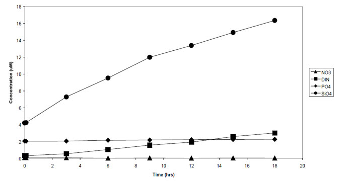
Figure 5.1. Change in nutrient concentrations with time, site 26.
Site 26
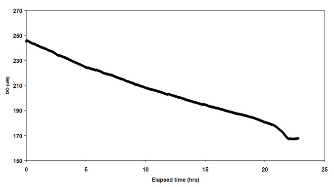
Figure 5.2. Change in dissolved oxygen concentration with time during incubation at site 26.
6.1 - Introduction
Within Australia, the use of video survey techniques for monitoring the impact of aquaculture has been developed mostly in Tasmania by the Tasmanian Aquaculture and Fisheries Institute and the Department of Primary Industry, Water and Environment. Video footage provides information on the distribution of native, farmed and introduced species. The footage also provides information on sediment colour and condition, including bioturbation by fauna and burrow density. On established aquaculture sites, video footage can also provide information on the presence of debris and shellfish accumulation under shell fish leases, and the presence of bacterial mats, food pellet and faeces accumulation under finfish enclosures.
For this study, a video survey of the benthic environment of the proposed Pinnace Channel Aquaculture Site was initiated to provide a visual record of the sea bed prior to the commencement of aquaculture activities, including information on sediment condition and the distribution and abundance of epifaunal species. Future surveys can use this footage to assess changes to epifaunal communities and sediment properties caused by aquaculture activities.
6.2 - Methods
The survey area has been described. Video transects were taken across each segment (Figure 2.1) using a video camera mounted on a sled and towed behind a small boat at less than two knots. The transects within each plot were aligned using a Differential GPS, offset 50 m to allow for the distance between the Differential GPS on the boat and the video sled trailing behind the boat. The width of the video transect was 1m. Video footage was recorded onto a Super VHS video recorder. On the video footage was included continuous information on latitude and longitude and speed over ground, from which the distance covered by the sled could be determined for any portion of footage.
Fifteen transects were originally proposed, but because of constraints imposed by time and weather video recordings were only made for nine transects (Figure 6.1). The video footage from these transects is stored on five, three-hour VHS tapes at MAFRI. Sections of six (of the 9) transects were analysed to determine the abundance of the dominant epifauna and to provide basic information on sediment type and condition. In total thirteen sections spread over the six transects were analysed. Five of the sections were from water less than 20 m in depth and 8 sections were from water of more than 20 m depth. As far as possible the sections chosen for analysis were those which were near to the sites of benthic stations chosen for analysis; but this was not possible for transect 15 since none of the benthic stations sorted for this phase of the project were close to transect 15. Analyses involved the use of a video player with a jog/shuttle function to slow-down the footage, where necessary, to allow identification of the fauna.
The composition and abundance of epifauna observed during this video survey are compared to the results obtained from surveys of epifauna carried out by divers in 1998 and 1999 at two 100 x 100m stations deliberately aligned over the proposed Pinnace Channel Aquaculture Site (Figure 6.1). Methods and results of this diver survey are reported in Cohen et al. (2000) and so are not described here.
6.3 - Results
Video footage distributed across six video transects (Figure 6.1) and covering approximately 5.5km of the seafloor was analysed for this study.
6.3.1 - Visual interpretation of sediments
Sediment characteristics and bottom relief varied across the surveyed area, mostly between sediments in water shallower than or deeper than 20m. Sediments in less than 20m of water were sandier than the sediments below 20m. The sandier sediment also supported large numbers of mounds and depressions caused by the bioturbation activity of Callianassid shrimps. These depressions collected large quantities of drift algae, which may have obscured the epibenthos present in these depressions. Depressions free of drift algae often contained large quantities of broken shell rubble. Occasional sparse Caulerpa beds, along with beds of an unidentified red alga, were also observed, indicating that the sediments were not highly mobile. Microalgal mats were not observed on these sandier sediments.
Sediments in greater than 20m of water were generally muddier, as indicated by the ease of disturbance by the video sled. The sediment surface profile was also more uniform than that observed on the sediments occurring in shallower water. Mounds and depressions caused by the bioturbation of Callianassid shrimps were generally absent, though numerous borrows were observed. Analysis of sediment granulometry (Chapter Three) confirmed that the percentages of mud and sand were respectively positively and negatively correlated with depth (Figure 3.1). Microalgal mats were not observed on the muddy sediments.
6.3.2 - Epifauna composition and abundance
Epifaunal species richness and abundances were low. Fourteen epifaunal species were identified from the video footage (Table 6.1). However, only 20 species were recorded by divers from the two stations used by Cohen et al. (2000) that are covered by the Pinnace Channel Aquaculture Site. The species lists across the two are very similar. The seven species recorded during the dive survey but not recorded on the video transects are all small or cryptic and would not be easily detected on video footage. Asterias amurensis, the introduced North Pacific seastar, is the only species not recorded by divers in 1998/99 that was recorded by the video survey.
The ascidian Pyura stolonifera was the most commonly recorded species on the video footage (670 individuals), followed by: oysters, Ostrea angasi (313); the introduced fan worm Sabella spallanzanii (156); the ascidian Cnemidocarpa etheridgii (128); and scallops, Pecten fumatus (58). All these species are filter feeders. The rank order of the most abundant species differed slightly to that observed by divers in 1998/99 (oysters, scallops, Pyura, Cnemidocarpa, Sabella).
Abundances of epifauna on the video footage were generally low, less than 10 individuals per 100m, with the exception of the ascidian Pyura stolonifera on sediments in less than 20m of water (Table 6.1). Abundances recorded during the video survey were generally lower than those recorded by the dive survey, although differences for most species were minimal. Scallops and oysters are sampled with much greater efficiency by divers than by video because both species are often shallowly buried and are therefore difficult to quantify accurately from video footage. Also, oysters are gregarious, growing on each other, and so are difficult to quantify accurately from the video footage. The abundance of the ascidian Pyura stolonifera in less than 20m of water, recorded on video footage, was much greater than that recorded by divers. The large standard error indicates that abundances of this species was very variable and that the different estimates of abundance obtained using the two different methods probably reflect the greater area covered by the video survey.
The abundance of many species varied between the shallow, sandy sediments and the deeper, muddy sediments. The sandy sediments, which generally occurred in waters less than 20m depth, supported significantly more of the ascidian Pyura stolonifera (ttest, P<0.0001). The muddier sediments, in water greater than about 20m, supported significantly more sea cucumbers Stichopus mollis (P=0.0005) and scallops (P=0.0141). These patterns are generally supported by the results observed from the dive survey (Table 6.1). The ascidian Cnemidocarpa etheridgii, the fan worm Sabella spallanzanii and oysters where more commonly encountered on the deeper, muddier sediments though differences were not statistically significant.
The video survey technique was also able to collect data on dermsal fish. Sand flathead were the most abundant fish (123 individuals), followed by stingarees (9), spikey globe fish, an unidentified toad fish and a spiny gurnard (1 of each). The area of the Pinnace Channel Aquaculture Site is not covered by the annual dermsal trawl survey conducted by MAFRI, though comparisons of similar sites would suggest that the Pinnace Channel Aquaculture Site fish community would be classified as part of the intermediate fish community according to Parry et al. (1995 - see also Cohen et al. 2000).
6.4 - Discussion
Epifaunal communities in Port Phillip have recently been classified by Cohen et al. (2000). Four communities were recognised. The region covered by the Pinnace Channel Aquaculture Site, including the Rye 17 and 22m sites used in the study by Cohen et al. (2000), is characterised by the 'intermediate sediments' epifaunal community (Figure 6.2). This epifaunal community comprises 34 species, the second highest species richness of the four Port Phillip Bay epifaunal communities. However, this community is also characterised by the lowest density of fauna and equally lowest biomass. It is unclear if this pattern is the result of recent scallop dredging activities or because of the proximity of this community to Port Phillip Heads and oceanic influences. The species distribution and abundance across the Pinnace Channel Aquaculture Site, recorded by the video survey, confirms that the composition of the epifaunal community is typical of the 'intermediate sediments' community. Asterias amurensis, the introduced North Pacific seastar, is the only species to be recorded by the video survey, which was not recorded by divers. The distribution of this species in Port Phillip Bay has expanded since its establishment in late 1997. Distribution and modelling work undertaken by MAFRI confirms that this starfish was absent or, at most, very rare around the Pinnace Channel Aquaculture Site during the summers of 1998 and 1999. However, it is not surprising to find low numbers of A. amurensis at the Pinnace Channel Aquaculture Site, given the current distribution of this species in Port Phillip.
Changes in the distribution and abundance of epifauna with depth occur across Port Phillip Bay. Cohen et al. (2000) observed a strong decrease in total abundance, biomass and species richness with depth and attributed this mostly to changes in the abundance of the ascidian Pyura stolonifera. Pyura is an important epibenthic species because it can act as an attachment site for other epibenthic species and provides refuge for mobile species. Pyura in Port Phillip Bay displays a preference for shallower, sandier sediments so it is not surprising to observe a marked decrease in the abundance of this species across the site between sediments above and below 20m. Differences in abundance observed between the video and diver survey probably reflect the greater accuracy of the method used by divers and the wider coverage of the video footage survey.
Whilst the purpose of the video survey was not a comparison between this method and the use of divers to survey epifaunal communities, both methods did give a similar picture of the epifauna of the proposed Pinnace Channel Aquaculture Site. That this is so generates confidence in the applicability video survey methods to monitor for any changes in the distribution and abundance of epifauna resulting from aquaculture activities. The advantage of the video method of survey is in the much larger area of coverage, compared to the method using divers, as divers are limited by the amount of dive time available, especially in the depths found across the Pinnace Channel Aquaculture Site.
Table 6.1: Mean abundance of fauna (±SE) per 100 x 1m transect surveyed by video sled, as part of the Pinnace Channel Baseline study, and by divers, as part of a study of Port Phillip Bay epifaunal communities (Cohen et al. 2000). Transect depths are in metres. For the Pinnace Channel data abundances are based on five analyses from water of less than 20 m depth and eight analyses from water of more than 20 m depth. For the diver transects, results are based on six transects at each depth.
| Species | Video transects | Diver transects | ||||
|---|---|---|---|---|---|---|
| Species | Depth | Mean | SE | Depth | Mean | SE |
| Ascidiella aspersa (exotic) |
< 20 > 20 |
0 0.05 |
0 0.05 |
17 22 |
0 4.00 |
0 3.06 |
| Halocynthia hispida |
< 20 > 20 |
0.05 0 |
0.05 0 |
17 22 |
0 1.33 |
0 0.88 |
| Pyura stolonifera |
< 20 > 20 |
0 0 |
0 0 |
17 22 |
0 1.33 |
0 0.88 |
| Herdmania momus |
< 20 > 20 |
0.70 0.49 |
0.24 0.15 |
17 22 |
1.00 1.00 |
1.00 0.63 |
| Styela clava (exotic) |
< 20 > 20 |
0 0.02 |
0 0.02 |
17 22 |
0 0.33 |
0 0.21 |
| Styela plicata (exotic) |
< 20 > 20 |
0.07 0 |
0.07 0 |
17 22 |
0 0.33 |
0 0.21 |
| Pyura irregularis |
< 20 > 20 |
0 0 |
0 0 |
17 22 |
0.66 1.33 |
0.49 0.66 |
| Cnemidocarpa etheridgii |
< 20 > 20 |
1.05 2.76 |
0.22 0.47 |
17 22 |
5.33 6.83 |
0.61 1.66 |
| Caberea cf. texta |
< 20 > 20 |
0 0 |
0 0 |
17 22 |
0.16 0 |
0.16 0 |
| Pilumnopeus serratifrons |
< 20 > 20 |
0 0 |
0 0 |
17 22 |
1.00 1.00 |
0.51 0.516 |
| Coscinasterias calamari |
< 20 > 20 |
0.33 0.27 |
0.22 0.10 |
17 22 |
0.16 0.50 |
0.16 0.34 |
| Tosia magnifica |
< 20 > 20 |
0.04 0 |
0.04 0 |
17 22 |
0 0.16 |
0 0.16 |
| Stichopus mollis |
< 20 > 20 |
0.04 0.67 |
0.04 0.30 |
17 22 |
0.66 2.66 |
0.21 1.22 |
| Asterias amurensis (exotic) |
< 20 > 20 |
0.50 0.08 |
0.50 0.05 |
17 22 |
0 0 |
0 0 |
| Mytilus edulis planulatus |
< 20 > 20 |
0 0 |
0 0 |
17 22 |
0.16 0.33 | 0.16 |
| Pterynotus triformis |
< 20 > 20 |
0 0 |
0 0 |
17 22 |
0 0.33 |
0 0.21 |
| Pecten fumatus |
< 20 > 20 |
0.48 2.03 |
0.36 1.24 |
17 22 |
13.66 25.16 |
3.52 6.62 |
| Ostrea angasi |
< 20 > 20 |
4.44 8.01 |
2.25 2.44 |
17 22 |
35.50 14.83 |
3.38 3.66 |
| Pleuroploca australasia |
< 20 > 20 |
0.11 0 |
0.11 0 |
17 22 |
0.16 0 |
0.16 0 |
| Anadara trapezia |
< 20 > 20 |
0 0 |
0 0 |
17 22 |
0.16 0 |
0.16 0 |
| Sabella spallanzanii (exotic) |
< 20 > 20 |
1.85 3.44 |
1.08 1.31 |
17 22 |
0 5.5 |
0 1.82 |
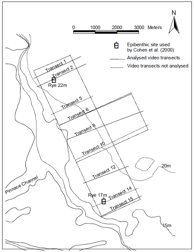
Figure 6.1. Pinnace Channel Aquaculture Site and location of the epibenthic transects sampled in the baseline survey of the area using a video sled. Video analyses were carried out for those transects shown as solid lines. Sites surveyed in 1998 and 1999 by divers as part of a Port Phillip Bay epibenthic survey are also marked (see Cohen et al. 2000).
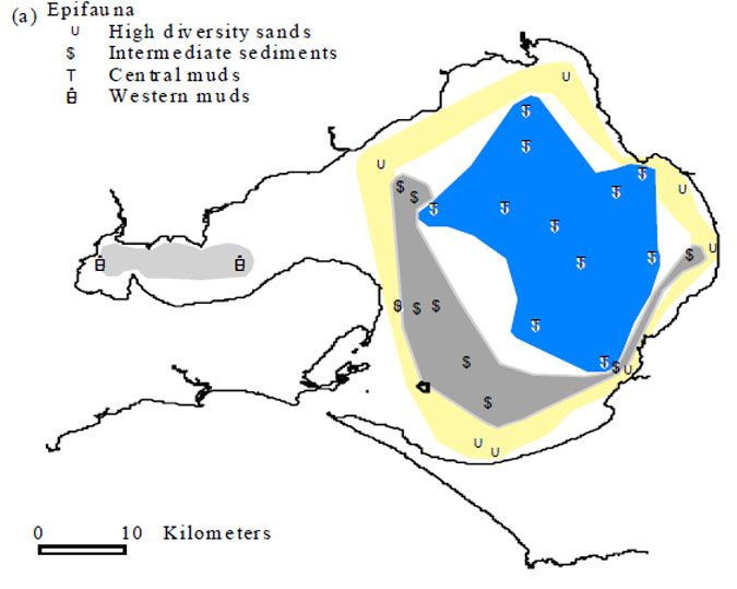
Figure 6.2. Map of Port Phillip Bay showing location of epifaunal stations and their classification into four communities based on MDS ordinations (see Cohen et al. 2000 Figure 5)
References
Figure 6.2. Map of Port Phillip Bay showing location of epifaunal stations and their classification into four communities based on MDS ordinations (see Cohen et al. 2000 Figure 5) REFERENCES
Atkinson, M.J. and Smith, S.V. (1983). C:N:P ratios in benthic marine plants. Limnology and Oceanography 28, 568-574.
Barry, J and Bailey, M. (2001). Bathymetric survey of the proposed aquaculture zone, Pinnace Channel, Port Phillip. Marine and Freshwater Resources Institute Internal Report No.?
Belbin, L. (1991). PATN pattern analysis program. Division of Wildlife and Ecology, CSIRO, Australia
Berelson, W.M., Heggie, D., Longmore, A., Kilgore, T., Nicholson, G. and Skyring,
G. (1998). Benthic nutrient recycling in Port Phillip Bay, Australia. Estuarine, Coastal and Shelf Science 46, 917-934.
Boon, P.I., Bird, F.L. and Bunn, S.E. (1997). Diet of the intertidal callianassid shrimps Biffarius arenosus and Trypea australiensis (Decapoda: Thalassinidea) in Western Port (southern Australia), determined with multiple stable-isotope analyses. Marine and Freshwater Research 48, 503-511.
Burke, C.M. (1999). Moelecular diffusive fluxes of oxygen in sediments of Port Phillip Bay in south-eastern Australia. Mar. Freshw. Res. 50, 557-566.
Cohen, B.F., Currie, D.R., and McArthur, M.A. (2000). Epibenthic community structure in Port Phillip Bay, Victoria, Australia. Marine and Freshwater Research 51, 689-702
CSIRO Huon Estuary Study Team. (2000). Huon Estuary Study. Environmental research for integrated catchment management and aquaculture. Project No. 96/284, FRDC. 285 pp.
Currie, D.R. and Parry, G.D. (1999). Changes to benthic communities over 20 years in Port Phillip Bay, Victoria, Australia. Marine Pollution. Bulletin 38(1), 36−43.
Dickson, A.G. (1981). An exact definition of total alkalinity and a procedure for the estimation of alkalinity and total inorganic carbon from titration data. Deep-Sea Research 28A, 609-623.
Fenton, G. and Ritz, D.A. (1988). Changes in carbon and hydrogen stable isotope ratios of macroalgae and seagrass during decomposition. Estuarine, Coastal and Shelf Science 26, 429-436.
France, R.L. (1995). Carbon-13 enrichment in benthic compared to planktonic algae: foodweb implications. Marine Ecology Progress Series 124, 307-312.
Fry, B. and Parker, P.L. (1979). Animal diet in Texas seagrass meadows: δ13C evidence for the importance of benthic plants. Estuarine and Coastal Marine Science 8, 499-509.
Fry, B., Scalan, R.S. and Parker, P.L. (1983). 13C/12C ratios in marine food webs of the Torres Strait, Queensland. Australian Journal of Marine and Freshwater Research 34, 707-715.
Fry, B. and Sherr, E.B. (1984). δ13C measurements as indicators of carbon flow in marine and freshwater ecosystems. Contributions in Marine Science 27, 13-47.
Fry, B. and Wainright, S.C. (1991). Diatom sources of 13C-rich carbon in marine food webs. Marine Ecology Progress Series 76, 149-157.
George, A.D. and Black, K.P. (1991). Settling tube analysis of sediment samples from eastern Bass Strait. Victorian Institute of Marine Sciences, Melbourne, Australia.
Gibbs, R.J., Matthews, M.D. and Link, D.A. (1971). The relationship between sphere size and settling velocity. Journal of Sedimimentary Petrology 41, 7−18
Gray, J.S., Clarke, K. R., Warwick, R.M. and Hobbs, G. (1990). Detection of initial effects of pollution on marine benthos: an example from the Ekofisk and Eldfisk oilfields, North Sea. Marine Ecology Progress Series 66, 2285 - 299.
Grice, A.M., Loneragan, N.R. and Dennison, W.C. (1996). Light intensity and the interactions between physiology, morphology and stable isotope ratios in five species of seagrass. Journal of Experimental Marine Biology and Ecology 195, 91-110.
Gu, B., Schelske, C.L. and Brenner, M. (1996). Relationship between sediment and plankton isotope ratios (δ13C and δ15N) and primary productivity in Florida lakes. Canadian Journal of Fisheries and Aquatic Sciences 53, 875-883.
Hansson, I. and Jagner, D. (1973). Evaluation of the accuracy of Gran plots by means of computer calculations. Application to the potentiometric titration of the total alkalinity and carbonate content in sea water. Analytica Chimica Acta 65, 363-373.
Harris, G., Batley, G., Fox, D., Hall, D., Jekanoff, P., Molloy, R., Murray, A., Newell, B., Parslow. J., Skyring, G. and Walker, S. (1996). Port Phillip Bay Environmental Study final report. CSIRO, Canberra.
Hemminga, M.A. and Mateo, M.A. (1996). Stable carbon isotopes in seagrasses: variability in ratios and use in ecological studies. Marine Ecology Progress Series 140, 285-298.
Henderson, A.R. and Ross, D.J. (1995). Use of macrobenthic infaunal communities in the monitoring and control of the impact of marine cage fish farming. Aquaculture Research 26, 659−678.
Hickman, N. and Coleman, N. (1998). Pinnace Channel Aquaculture Area in Port Phillip Bay. Site characterisation and summary of background environmental information and monitoring capability. Marine and Frehwater Resources Institute.
Hobson, K.A., Ambrose, W.G. Jr. and Renaud, P.E. (1995). Sources of primary production, benthic-pelagic coupling, and trophic relationships within the Northeast Water Polynya: insights from δ13C and δ15N analysis. Marine Ecology Progress Series 128, 1-10.
Ismail, N. (1992). Macrobenthic invertebrates near sewer outlets in Dubai Creek, Arabian Gulf. Marine Pollution Bulletin 24, 77−81.
Kaiser, M.J., Laing, I., Utting, S.D. and Burnell, G.M. (1998). Environmental impacts of bivalve mariculture. Journal of Shellfish Research 17(1), 59−66.
Loneragan, N.R., Bunn, S.E.and Kellaway, D.M. (1997). Are mangroves and seagrasses sources of organic carbon for penaeid prawns in a tropical Australian estuary? A multiple stable-isotope study. Marine Biology 130, 289-300.
Longmore, A.R. (2000). Port Phillip Bay nutrient monitoring proposal- scientific and technical advice. MAFRI Report No. 16. 51 pp.
Longmore, A.R., Cowdell, R.A. and Flint, R. (1996). Nutrient status of the water in Port Phillip Bay. CSIRO Port Phillip Bay Environmental Study Technical Report No. 24, Melbourne.
Longmore, A.R. and Gason, A. (2001). Port Phillip Bay nitrogen monitoring proposal- statistical advice. MAFRI Report No. 32. 49 pp.
Nichols, P.D., Klumpp, D.W., and Johns, R.B. (1985). A study of food chains in seagrass communities III. Stable carbon isotope ratios. Australian Journal of Marine and Freshwater Research 36, 683-690.
Nicholson, G.J, Longmore, A.R. and Berelson, W.M. (1999). Nutrient fluxes measured by two types of benthic chamber. Marine and Freshwater Research 50, 567−572.
Parry, G.D., Hobday,D.K., Currie, D.P., Officer, R.A. and Gason, A.S. (1995) The distribution, abundance and diets of demersal fish in Port Phillip Bay. CSIRO Port Phillip Bay Environmental Study Technical Report No. 21, Melbourne.
Parsons, T.R., Maita, Y. and Lalli, C.M. (1984). A manual of chemical and biological methods for seawater analysis. Pergamon Press, Oxford, UK.
Pearson, T. H. and Rosenberg, R. (1978). Macrobenthic succession in relation to organic enrichment and pollution of the marine environment. Oceanography and Marine Biology Annual Review 16, 229−311
Poore, G.C.B. (1992). Soft-bottom macrobenthos of Port Phillip Bay:a literature review. Technical Report No. 2. CSIRO Port Phillip Bay Environmental Study. Melbourne. 24 pp Poore, G.C.B., Rainer, S.F., Spies, R.B. and Ward, E. (1975) The zoobenthos program in Port Phillip Bay, 1969-73. Fisheries and Wildlife Paper, Victoria No. 7. Fisheries and Wildlife Division, Victoria, Australia.
Santschi, P., Hohener, P., Benoit, G. and Buchholtz-ten Brink, M. (1990). Chemical processes at the sediment-water interface. Marine Chemistry 30, 269-315.
Swartz, R.C., Cole, F. A., Schults, D.W. and DeBen, W.A. (1986). Ecological changes in the Southern California Bight near a large sewage outfall: benthic conditions in 1980 and 1983. Marine Ecology Progress Series 13, 1−13
Sweeney, R.E. and Kaplan, I.R. (1980). Natural abundances of 15N as a source indicator for near-shore marine sedimentary and dissolved nitrogen. Marine Chemistry 9, 81-94.
Wilson, R.S., Heislers, S.I. and Poore, G.C.B. (1998). Changes in benthic communities of Port Phillip Bay, Australia, between 1969 and 1995. Marine and Freshwater Research 49, 847−861.
Zarkanellas, A.J. (1979). The effects of pollution-induced oxygen deficiency on the benthos in Elefsis Bay, Greece. Marine Environmental Research 3, 191−207.